Back to Blog January 14, 2026
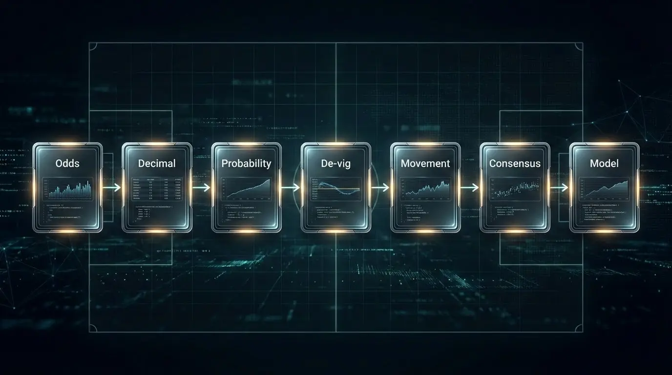
InsightsJanuary 14, 20268 min read
Inside Our Feature Pipeline: How Raw Data Becomes Prediction Input
A look at how we transform raw market data into structured features—probability normalization, movement signals, consensus metrics, and cross-market validation.
OddsFlow Team
OddsFlow Team
#feature engineering#machine learning pipeline#data transformation#AI predictions#sports analytics#data science